I set out to do a project using my learnings from the first chapter of the fast.ai course. My first idea was to try and train a Ruby/Python classifier. ResNets are not designed to do this, but I was curious how well it would perform.
Classifying images of sources code by language
My first idea was to download a bunch of source code from GitHub, sort it by language type, then convert it to images with Carbon. After working through some GitHub rate limiting issues, I eventually had a list of the top 10 repositories for several different languages. From here, I created a list of files in these repos, filtering by the extension of the programming language I wanted to download.
At this point, I was a bit irritated dealing with the GitHub API, and though I was actually close to building the dataset, I had another idea.
I wrote some more code to use gpt-4o-mini to generate 100 files of both Python and Ruby source code.
def generate_code(language):
    response = client.chat.completions.create(
        model="gpt-4o-mini",
        messages=[
            {"role": "user", "content": f"write a some very realistic looking code in {language}. output code and code only. do not use code fences"}
        ],
        temperature=1.4,
    )

    return response.choices[0].message.content
Next, I used the carbon-now-cli to create images of the source code the model generated.
I set up a few different color presets for variety.
import subprocess
import os
import random

generated_code_path = os.path.join(os.getcwd(), "generated_code")

styles = [
    "hacker",
    "presentation",
    "matrix",
    "neon",
    "cyberpunk",
]

for language in languages:
    folder_path = os.path.join(generated_code_path, language)

    for file_name in os.listdir(folder_path):
        file_path = os.path.join(folder_path, file_name)
        style = random.choice(styles)

        try:
            command = f"npx carbon-now-cli {file_path} --save-to images/{language} -p {style}"
            result = subprocess.run(command, shell=True, check=True, capture_output=True, text=True)
        except subprocess.CalledProcessError as e:
            print(f"Error processing file {file_name}: {e}")
Once I had the images in their respective language folders, I wrote fastai code to finetune a model.
from fastcore.all import *
from fastai.vision.all import *

path = Path('images')
dls = DataBlock(
    blocks=(ImageBlock, CategoryBlock),
    get_items=get_image_files,
    splitter=RandomSplitter(valid_pct=0.2, seed=42),
    get_y=parent_label,
    item_tfms=[Resize(1024, method='squish')]
).dataloaders(path, bs=32)
Finetune the model
learn = vision_learner(dls, resnet18, metrics=error_rate)
learn.fine_tune(3)
Once the training was finished, I took a screenshot of some Python code I had locally and downloaded an image of Ruby from online. The model classified both images as Ruby with very high confidence. I also tried running some of the images from the training data through the model. For these, it identified the Python code correctly. The model seemed to have memorized the training data but didn’t identify patterns to effectively generalize.
Introducing Java to the mix
To see what would happen, I generated 100 files of Java source code, then converted those to images. I trained the same model on the original ~200 Python and Ruby code images plus the additional 100 Java code images. Once trained, I tried the same tests again. The model continued identifying all code as Ruby.
Removing Python
Python and Ruby look quite similar, so I tried removing the Python images from the training data and just trained on the Ruby and Java images. I still ran into the same problem. The model was identifying the Java source code as Ruby. I even took a screenshot of a subset of an image of Java code used in the training data. The model still spit out Ruby.
Trying a different model
Out of ideas of things to try with the data for the time being, I decided to try a different model.
I picked resnet50 from this list because I don’t know any better.
It was taking a while to train, so I walked away for a while.
Here are the results
Extracted by pasting an image of the table from the notebook into a Cursor/Sonnet prompt
from training the resnet50 model:
| epoch | train_loss | valid_loss | error_rate | time |
|---|---|---|---|---|
| 0 | 0.381366 | 0.679645 | 0.365854 | 05:26 |
| 1 | 0.250793 | 0.250266 | 0.073171 | 05:59 |
| 2 | 0.185864 | 0.125285 | 0.048780 | 04:42 |
The error rate was lower than the resnet18 model (didn’t copy these over), but was the model actually functional?
It didn’t seem to be.
It got none of my test images correct.
Then I remembered fastai has a way to run the test set on the model, that it sets aside during training.
Or at least I thought it did.
I couldn’t find anything referencing a test set in the chapter 1 or lecture notebooks.
I also checked the lesson 1 transcript with a script I added as a variation to my YouTube video summarization script.
I was reminded that test datasets are important, but it seems the lesson material didn’t cover this yet.
I decided not to dig too far ahead for this part.
Generating more synthetic data
While my realistic examples didn’t work, I figured it was at least worth trying to generate a few more images from synthetic data, following the same process to see how the model performed. This actually worked well! In retrospect, it kind of makes sense. I only trained on 5 different color schemes and using images generated by the same process likely biased the training to those specific types of images and not those I downloaded or created from screenshots. If I wanted this to work better, I probably would need to train it on a more diverse set of screenshots.
Classifying voices by spectrograms images of audio
Because I didn’t quite get the source code example working, I decided to try something else.
I used the macOS command say to render short audio snippets of two different system voices (Samantha and Evan), then tried to train an image model of the spectrograms of each audio segment to see if I could identify which voice was speaking.
I used the following code to generate the audio files:
import subprocess

def create_aiff_file(voice, text, output_filename):
    output_path = os.path.join(audio_folder, voice, output_filename)

    command = [
        'say',
        '-v', voice,
        '-o', output_path,
        text
    ]

    try:
        subprocess.run(command, check=True, capture_output=True, text=True)
        return output_path
    except subprocess.CalledProcessError as e:
        return None
Next, I used this code to generate the spectrograms:
import librosa
import librosa.display
import matplotlib.pyplot as plt
import numpy as np

def create_spectrogram(input_file, output_file):
    y, sr = librosa.load(input_file)
    S = librosa.feature.melspectrogram(y=y, sr=sr, n_mels=128, fmax=8000)
    S_dB = librosa.power_to_db(S, ref=np.max)
    plt.figure(figsize=(12, 8))
    librosa.display.specshow(S_dB, cmap='viridis')
    plt.axis('off')
    plt.gca().set_position([0, 0, 1, 1])
    plt.savefig(output_file, dpi=300, bbox_inches='tight', pad_inches=0)

    plt.close()
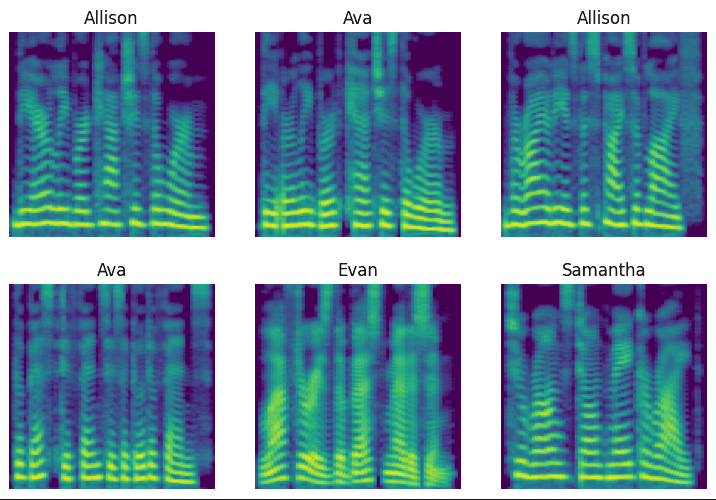
Here is what these images looked like (this is an example from later when I was using 4 different voices):
This didn’t seem to work at all – even less well than the programming language classification.
I tried a few different approaches at creating visuals from the audio files but none seemed to work.
I only had 25 examples though, so I decided to create some more data to see if that could help.
I generated another 75 examples
Visual inspection of the labeled images in the Datablock didn’t reveal any obvious difference between the two voices, so I was relying on some model magic to happen with the finetuning
per voice then trained resnet34 again.
learn = vision_learner(dls, resnet34, metrics=error_rate)
learn.fine_tune(5)
These were the training stats:
| epoch | train_loss | valid_loss | error_rate | time |
|---|---|---|---|---|
| 0 | 0.391036 | 0.955989 | 0.461538 | 00:33 |
| 1 | 0.249562 | 0.801549 | 0.384615 | 00:33 |
| 2 | 0.181186 | 0.321640 | 0.153846 | 00:32 |
| 3 | 0.138594 | 0.184952 | 0.076923 | 00:32 |
| 4 | 0.114745 | 0.121491 | 0.051282 | 00:32 |
This time it worked pretty well! It got 4/4 of my tests correct with high accuracy.
Introducing more voices
Finally with some success, I decided to try to introduce a few more voices (Ava and Allison) to see if I could classify all four effectively with 100 examples of each and the same model architecture. Training took a bit longer with a doubling of the amount of training data. These were the training results:
| epoch | train_loss | valid_loss | error_rate | time |
|---|---|---|---|---|
| 0 | 0.685900 | 0.776896 | 0.253165 | 01:06 |
| 1 | 0.390314 | 0.473427 | 0.126582 | 01:07 |
| 2 | 0.250393 | 0.252311 | 0.075949 | 01:06 |
| 3 | 0.179241 | 0.205531 | 0.050633 | 01:06 |
| 4 | 0.131612 | 0.164919 | 0.050633 | 01:05 |
I tried 8 test examples, 2 of each voice. The model got 8/8 correct!
('Evan', tensor(2), tensor([2.3281e-05, 3.3971e-05, 9.9991e-01, 3.5356e-05]))
('Evan', tensor(2), tensor([1.0040e-03, 8.6804e-04, 9.9276e-01, 5.3682e-03]))
('Samantha', tensor(3), tensor([3.4169e-03, 4.2099e-04, 3.9679e-06, 9.9616e-01]))
('Samantha', tensor(3), tensor([0.0362, 0.0993, 0.0745, 0.7901]))
('Ava', tensor(1), tensor([2.3982e-04, 9.9952e-01, 9.1395e-06, 2.2789e-04]))
('Ava', tensor(1), tensor([5.3671e-04, 9.9940e-01, 2.5800e-05, 3.7564e-05]))
('Allison', tensor(0), tensor([9.7594e-01, 2.3934e-02, 1.2181e-05, 1.0872e-04]))
('Allison', tensor(0), tensor([9.9855e-01, 1.2605e-04, 2.2478e-06, 1.3212e-03]))
This experiment was a success! It was quite cool to see something finally working.
Trying a smaller model
With my nice example finetuned on resnet34, I tried the same process on resnet18 to see if the smaller model architecture could perform as well.
learn = vision_learner(dls, resnet18, metrics=error_rate)
learn.fine_tune(5)
Training seemed to take about as long (around 5 minutes).
Here are the training results for the smaller model (resnet18):
| epoch | train_loss | valid_loss | error_rate | time |
|---|---|---|---|---|
| 0 | 0.641440 | 0.961596 | 0.430380 | 01:02 |
| 1 | 0.416878 | 0.264568 | 0.063291 | 01:03 |
| 2 | 0.275593 | 0.207364 | 0.037975 | 01:02 |
| 3 | 0.197330 | 0.159479 | 0.037975 | 01:01 |
| 4 | 0.146463 | 0.151528 | 0.050633 | 01:02 |
The smaller model (resnet18) performed similarly to the larger model (resnet34), achieving comparable error rates in about the same amount of time. The results were just as good!
('Evan', tensor(2), tensor([1.1675e-06, 9.1775e-07, 9.9998e-01, 1.5757e-05]))
('Evan', tensor(2), tensor([3.9756e-04, 8.6323e-05, 9.9935e-01, 1.7035e-04]))
('Samantha', tensor(3), tensor([1.4443e-04, 6.6675e-05, 6.8908e-05, 9.9972e-01]))
('Samantha', tensor(3), tensor([0.2441, 0.1274, 0.0844, 0.5440]))
('Ava', tensor(1), tensor([0.0019, 0.9748, 0.0026, 0.0207]))
('Ava', tensor(1), tensor([1.6715e-03, 9.9817e-01, 1.4240e-04, 1.4866e-05]))
('Allison', tensor(0), tensor([9.9991e-01, 8.5184e-05, 3.1841e-07, 2.0744e-06]))
Takeaways
- If a model’s loss isn’t decreasing, it can help to train on more data.
- Withholding a test set is necessary so that you can systematically see if what you built is any good at generalizing after training.
- A bigger model doesn’t necessarily perform better.
- A smaller model doesn’t always train faster.
- Making clean (sharable) notebooks isn’t easy but is something I want to get better at (due to this and time constraints, I probably won’t have the notebooks I used for this work available for a little while).
- The speed at which I can work through these experiments and learn ML is aided significantly by help from Sonnet writing code to do dataset generation. Doing this was most of the work, but I was able to pivot away from generating images of source code and to generated spectrograms of audio quite quickly compared to needing to write all the code from scratch myself. I might have stopped completely after the first attempt had it not been for LLM codegen and I wouldn’t have completed the most interesting part.
- It’s easy to leave a bunch of Jupyter Kernels running which can take over your system’s memory. By the end of this experiment, I had 4 separate python processes running, using between 56 and 68 GB of memory. At this point, my system tapped out and I had to manually clean these up.
- The numbers in model architecture names (e.g. the 34 in
resnet34compared to the 19 invgg19_bn) should not be used to compare relative sizes between different model architecture families. However, within the same family, these numbers often indicate relative depth or complexity. For example,resnet34has more layers thanresnet18.